Just when you think you have a good “recipe” to process astronomy images taken with your gear, things don’t quite work out and you end up spending three evenings trying different settings, techniques and steps because you know there’s a better image waiting to be teased out.

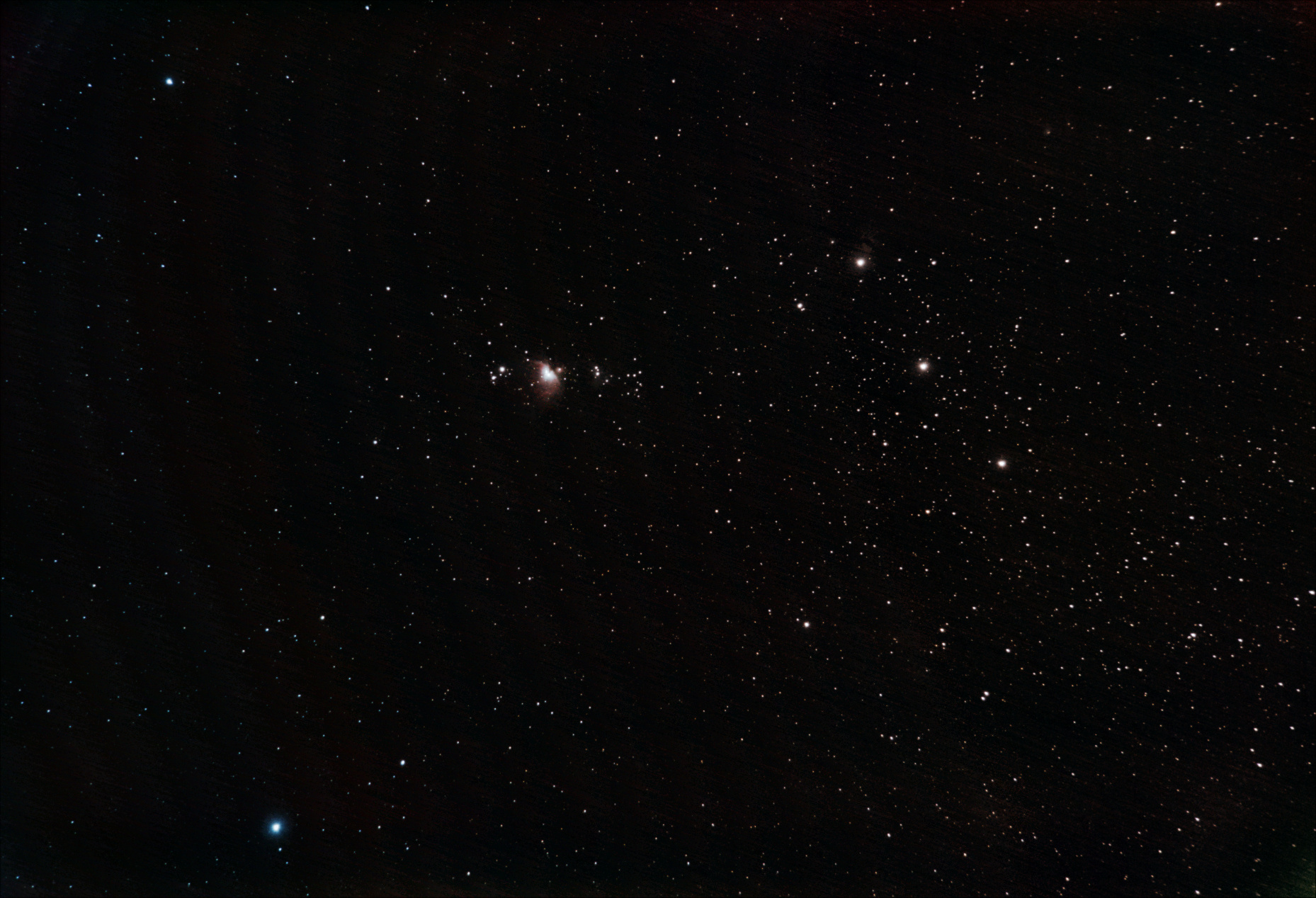
M72 and Lower Orion Constellation – Benoit Guertin

The image above (click for a full frame) is as much as I can stretch out from the lower half  of the Orion constellation and nebula with a 20 seconds ISO 800 exposure on 85mm F5.6 Canon lens from my light polluted backyard.

Below is the sky chart of the same area showing the famous Orion Nebula (blue and red box) and the Orion belt with the three bright stars Alnitak, Alnilam and Mintaka.  What is unfortunate is there are lots of interesting deep space nebula structures that glow in the hydrogen-alpha spectral lines of near infra-red, but all photographic cameras have IR filters to cut on the sensor those out.  That is why many modify the cameras to remove the filter, or get dedicated astro-imaging cameras.

Sky Chart – Lower Orion with nebula and open star clusters

Now, back to the main topic of trying to process this wide field image.  I had various issues with getting the background sky uniform, other times the color just disappeared and I was left with essentially a grey nebula; the distinctive red and greenish hue from the hydrogen and oxygen molecules was gone.  And there was the constant hassle of removing noise from the image as I was stretching it a fair bit.  I also had to be careful as I was using different software tools, and each don’t read/write the image files the same way.  And some formats would cause bad re-sampling or clipping, killing the dynamic range.

Below is a single 20 seconds exposure at ISO 800.  The Orion nebula (M72) is just barely visible over the light pollution.

Original image – high light position for 20 seconds exposure

The sky-flog (light pollution) is already half way into the light levels.  Yes, there are also utility lines in the frame.  As these will slightly “move” with every shot as as the equatorial mount tracked I figured I could make them numerically disappear.  More on that later…

Light levels of a 20 second exposure due to “sky fog”

The longer you expose, the more light enters the camera and fainter details can be captured.  However when the background level is already causing a peak mid-way, longer exposures won’t give you fainter details; it will simply give you a brighter light-polluted background.  So I needed to go with quantity of exposures to ideally reach at least 30 minutes of exposure time. Therefore programmed for 100 exposures.

Once the 100 exposures completed, I finished with dark, flat and offset frames to help with the processing.  So what were the final steps to reach the above final result?   As mentioned above, I used three different software tools, each for a specific set of tasks: DSS for registration and stacking, IRIS for color calibration and gradient removal and finally GIMP for levels and noise removal.

1. Load the light, dark, flats and offset images in Deep Sky Stacker (DSS).
2. Perform registration and stacking.  To get rid of the utility lines as well as any satellite or airplane tracks, the Median Kappa-Sigma method to stack yields the best results.  Essentially anything that falls out of the norm gets replaced with the norm.  So aircraft navigation lights which show up only on one frame of 100 gets replaced with the average of all the other frames.  That also meant the utility lines, which moved at every frame due to the mount tracking, would vanish in the final result.
3. As my plan is to use IRIS to calibrate colors, where I can select a specific star for the calibration, I set the no background or RGB color calibration for DSS.
4. The resulting file from DSS is saved in 16-bit TIF format (by default DSS saves in 32-bit, but that can’t be opened by IRIS).  I didn’t play around with the levels or curves in DSS.  That will be dealt later, a bit in IRIS, but mostly in GIMP.
5. I use IRIS to perform background sky calibration to black by selecting the darkest part of the image and using the “black” command.  This will offset each RGB channel to read ZERO for the portion of the sky I selected.  The reason for this is the next steps work best when a black is truly ZERO.  While IRIS works in 16-bit, it’s actually -32,768 to + 32,768 for each RGB channel.  If your “black” has an intensity of -3404, the color calibration and scaling won’t be good.
6. The next step requires you to find a yellow Sun-like star to perform color calibration.  As a white piece of paper under direct sunlight is “white”, finding a star with similar spectral color is best.  Sky chart software can help you with that (Carte du Ciel or C2A is what I use).  Once located and selected the “white” command will scale the RGB channels accordingly.
7. The final step is to remove the remaining sky gradient, so that the background can be uniform.  Below is the image before using the sky gradient removal tool in IRIS.

8. 

   Image before removal of sky gradient in IRIS

9. Once the sky gradient is removed, the tasks in IRIS is complete, save the file in BMP format (will be 16-bit)  for the next software: GIMP
10. The first step in GIMP is to adjust light curves and levels.  This is done before any of the filers or layer techniques is performed.
11. Then I played around with the saturation and Gaussian blur for noise reduction.  As you don’t always want the transformations to take place on the entire image, using layers is a must.
12. For the final image above, I created two duplicate layers, where I could play with color saturation, blurring (to remove the background noise) and levels until I got the desired end result.  Masks are very helpful in selecting what portion of the image should be transparent to the other layers.  An example is I wanted a strong blur to blend away the digital image processing noise, but don’t want a final blurry night sky.